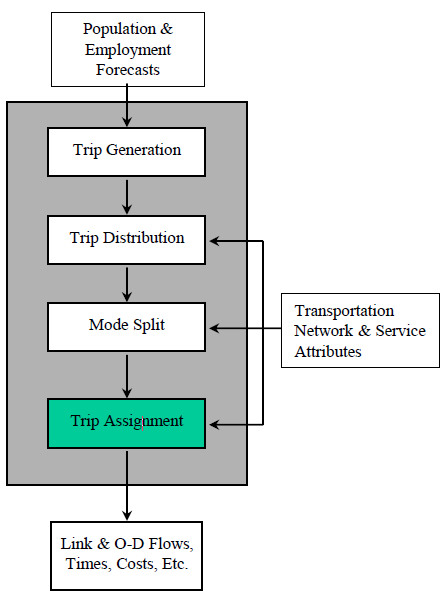
Lecture 7 - Trip Assignment
CIVE 461/861: Urban Transportation Planning
Outline
- Problem definition & assumptions
- Shortest path algorithms
- Representing congestion
- Treatment of time
- Random effects
- Wardrop’s rules: System optimal & User equilibrium
- Assignment procedures: All-or-nothing, Capacity restraint, & Deterministic user equilibrium
Trip Assignment Problem
- Find the path (or paths) through the network mostly likely taken from node i to node j
- Transport network is represented by links L
- Each link has a start & end node, as well as a cost C
- Links can also be mode-specific (e.g., bus-only, bus & vehicles)
- Link cost is a function of attributes: distance, free-flow speed, capacity, & speed-flow relationship (volume-delay function)
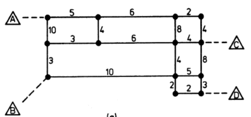
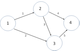
Shortest Path Example
What is the shortest path from Node 6 to All Others?

Shortest Path Example
Step 3: Find neighbors of current node Node 6 neigbors: {1,4,5}
Step 4: Update tentative costs
| Node pair | Cost (previous cost) |
|---|---|
| 6,1 | 5 (infinity) |
| 6,4 | 3 (infinity) |
| 6,5 | 8 (infinity) |
Costs are less than previous, so update table
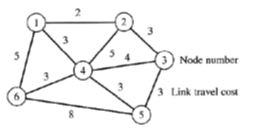
Shortest Path Example

Congestion Effects
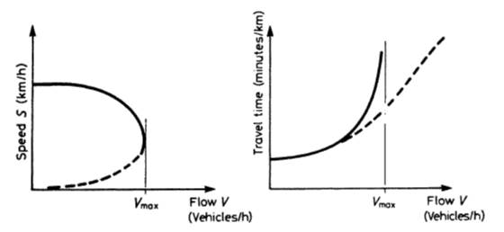
- On most urban road networks, congestion effects are significant (especially during peak periods)
- Generally, use volume-delay curve to predict link travel time (t) as function of link volume (v)
- Volume-delay functions are simple approximations to true link performance
Volume-Delay Function: Supply Curve/Performance Function

Example BPR Function

Deterministic Vs. Stochastic Assignment
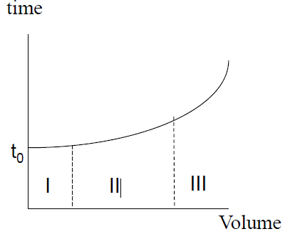
- I: in fairly uncongested condition as network is going towards saturation. Deterministic & stochastic assignment work in same way
- II: Congestion building up & deterministic approach will under-estimate effect.
- Stochastic assignment is better.
- III: Highly congested situation, small increase in volume causes larger increase in time.
- Penalty for wrong information would incur high delay. Assuming users aware of situation, deterministic assignment more appropriate.
All-Or-Nothing Assignment: Example
OD trips to be assigned:
A-C = 400
A-D = 200
B-C = 300
B-D = 100
- Find shortest paths for A-D, A-C, B-C, & B-D
- Assign all trips to corresponding shortest paths
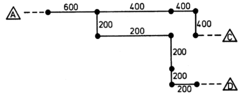
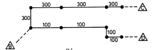
All-Or-Nothing Assignment: Example
Sum all assigned trips to get complete assignment

Incremental Assignment Methods

Incremental Assignment: Example
\[t_1 = \frac{t_{01}}{1-v_1/c_1}\] where:
\(t_1\) = travel time on link 1
\(t_{01}\) = travel time on link 1 under zero flow condition
\(v_1\) = volume on link 1
\(c_1\) = capacity of link 1
| Link | 1 | 2 | 3 | 4 | 5 |
|---|---|---|---|---|---|
| \(T_0\) | 10 | 15 | 3 | 5 | 4 |
| Capacity | 300 | 500 | 150 | 200 | 200 |
O-D trips to assign:
| From/To | 1 | 2 | 3 | 4 |
|---|---|---|---|---|
| 1 | 0 | 100 | 100 | 100 |
| 2 | 0 | 0 | 50 | 50 |
| 3 | 0 | 0 | 0 | 100 |
| 4 | 0 | 0 | 0 | 0 |
Random assignment order:
| To | ||
|---|---|---|
| O-D Pair | 1 | 2 |
| (1,2) | 1 | 3 |
| (1,3) | 6 | 6 |
| (1,4) | 2 | 4 |
| (2,3) | 3 | 2 |
| (2,4) | 5 | 5 |
| (3,4 | 4 | 1 |
Capacity Constrained Deterministic User Equilibrium (DUE)
- Note the two routes between same O-D pair will be used by trip-makers iff the travel times on the two routes are the same.
- Consider a single O-D pair (origin A & destination B) with two links (routes) connection them (1 & 2)

Volume-Delay Functions (VDF) for Links 1 & 2

Equilibrium Solution
- Special case: curves may not intersect
- Here, optimum is area under \(f_2(v_2)\)
![]()

Frank-Wolfe Algorithm
- Equilibrium link volumes are such that the sum of the areas under the volume-delay curves equals the minimum value achievable:
- F(V) given by \[min \sum_l \int_0^{v_l}f_l(v) d(v) \text{ (𝐸𝑄1)}\]
- Above equation generalizes to any number of O-D pairs & any number of links per path

Frank-Wolfe Algorithm

Frank-Wolfe Algorithm
